• Skip to main content
  • Skip to footer
Revelwood Logo

Revelwood

Your SUPER-powered WP Engine Site

  • Who We Are
    • About Us
      • Our Company
      • Our Team
      • Partners
    • Careers
      • Join Our Team
  • What We Do
    • Solutions
      • Workday Adaptive Planning
      • IBM Planning Analytics
      • BlackLine
    • Services
      • Implementation Services
      • Customer Care
        • Help Desk
        • System Administration as a Service
      • Training
        • Workday Adaptive Planning Training
        • IBM Planning Analytics / TM1 Training
    • Products
      • DataMaestro
      • LightSpeed
      • IBM Planning Analytics Utilities
  • How We Help
    • Use Cases
    • Client Success Stories
  • How We Think
    • Knowledge Center
    • Events
    • News
  • Contact Us

Excel tips & tricks

IBM Planning Analytics Tips & Tricks: Excel Keyboard Navigation

January 5, 2021 by Lee Lazarow Leave a Comment

Have you ever wanted to quickly go to the last used cell within a spreadsheet but did not know how? Have you ever wanted to determine where the next available row or column resides? Have you ever wondered why a spreadsheet with only a few cells of data may appear as a large file? All these answers can be provided with a single keystroke combination.

Pressing Ctrl and End at the same time will bring you to the last cell within a spreadsheet that Excel is referencing. The definition of “last” entails the rightmost column and the lowest used row on the worksheet. The last cell may not always contain data, but it will always be registered by Excel as something that is utilizing memory.

Here are some other keystroke combinations that will help you quickly navigate around your spreadsheet:

  • Ctrl and Home at the same time: this will bring you to the first cell (A1) in the worksheet.
  • End then an arrow key: this will bring you to the next empty value in any direction. For example, pressing End and then the down arrow will bring you to next empty cell in the column where your cursor currently resides.
  • Ctrl and PageUp : this will bring you to the previous sheet in the workbook.
  • Ctrl and PageDn: this will bring you to the next sheet in the workbook.

Keyboard shortcuts can easily help you navigate your Excel files and help you determine the “ending” cell within a spreadsheet.  This will be useful in situations such as dynamic reports where rows and columns are automatically generated via automation.

IBM Planning Analytics, which TM1 is the engine for, is full of new features and functionality. Not sure where to start? Our team here at Revelwood can help. Contact us for more information at info@revelwood.com. And stay tuned for more Planning Analytics Tips & Tricks weekly in our Knowledge Center and in upcoming newsletters!

Read more Excel Tips & Tricks:

IBM Planning Analytics Tips & Tricks: Learn the Excel CELL Formula

IBM Planning Analytics Tips & Tricks: Excel’s IFS Function

IBM Planning Analytics Tips & Tricks: Excel LET Function

Home » Excel tips & tricks » Page 2

Filed Under: IBM Planning Analytics Tips & Tricks Tagged With: enterprise performance management, Excel, Excel tips & tricks, Financial Performance Management, IBM Cognos TM1, IBM Planning Analytics, lee lazarow, Planning Analytics tips, Planning Analytics Tips & Tricks, Revelwood, TM1

IBM Planning Analytics Tips & Tricks: Excel LET Function

September 8, 2020 by Lee Lazarow Leave a Comment

Have you ever created a formula that repeats another formula within a cell? Did you know that this repetition may be slowing down your reports?

For example, you may have a report where you want to pull IBM Planning Analytics data and replace zeros with the word “None.”  You can write this as a formula via:

=IF ( DBRW(cube,dim1,dim2,dim3)=0, “None”, DBRW(cube,dim1,dim2,dim3) )

Within this formula, the IF check first looks at the DBRW formula to determine a value. If the value is not zero then the IF check needs to re-run the exact same DBRW formula to produce the value that will appear in the cell.  This means that one cell potentially needs to run the same formula twice! While this doesn’t sound like a big deal, it can easily impact the performance of your report if you have many iterations of the formula.

Excel has introduced a new function called LET that will help optimize this situation. This function allows you to define a variable that can repeatedly be used within a calculation. It will help you improve performance since it will only execute the calculation once within the cell.

The syntax of the function is:

=LET (VarName, VarValue, Calculation)
  • VarName is the name of the variable to be used
  • VarValue is the value of the variable
    • This can be a hard coded number or it can be a formula
  • Calculation is a formula that uses the variable name
    • This can be a simple formula such as X+Y or it can use any existing Excel function

A simple iteration of this formula can be written as:

=LET (x, 5, x*2)

This formula would result in the number 10.

The LET formula also allows you to define multiple variables.  A simple example of multiple variables can be written as:

=LET (x, 5, y, 2, x*y)

This formula would also result in the number 10.

Using this approach, our initial formula can be rewritten using the LET function:

=LET ( CubeVal, DBRW(cube,dim1,dim2,dim3), IF(CubeVal=0,”None”, CubeVal) )

This ensures that the DBRW pull is only executed once within the cell.

This functionality allows you to optimize your Excel based reports by minimizing the number of calculations that happen within your report.

IBM Planning Analytics, which TM1 is the engine for, is full of new features and functionality. Not sure where to start? Our team here at Revelwood can help. Contact us for more information at info@revelwood.com. And stay tuned for more Planning Analytics Tips & Tricks weekly in our Knowledge Center and in upcoming newsletters!

Read more Excel Tips & Tricks:

IBM Planning Analytics Tips & Tricks: Learn the Excel CELL Formula

IBM Planning Analytics Tips & Tricks: The Excel FORMULATEXT Function

IBM Planning Analytics Tips & Tricks: New Excel Feature – XLOOKUP

 
Home » Excel tips & tricks » Page 2

Filed Under: IBM Planning Analytics Tips & Tricks Tagged With: Analytics, Excel tips & tricks, Financial Performance Management, IBM Cognos TM1, IBM Planning Analytics, Planning Analytics tips, Planning Analytics Tips & Tricks, TM1

IBM Planning Analytics Tips & Tricks: Excel’s FILTER Function

June 23, 2020 by Lee Lazarow Leave a Comment

Tips & Tricks

Have you ever wanted to filter a list of data to look at a subset of the entire table? Many of you know that you can use the filter button within Excel’s data section to do this.

IBM Planning Analytics Tips & Tricks: The Excel FILTER Function

But what if you wanted to create a filter that users can change without having to navigate through ribbons? Did you know that you can do this using Excel’s FILTER function?

The FILTER function allows you to filter a range of data based on criteria you define. This allows you to create selector cells which can be used within a formula to filter the selected data. The function is written as follows:

FILTER (range, formula for inclusion, if empty)

  • The range consists of the entire table to be checked
  • The formula for inclusion consists of criteria to be filtered
  • The last parameter (optional) defines a value to be returned when no results are found

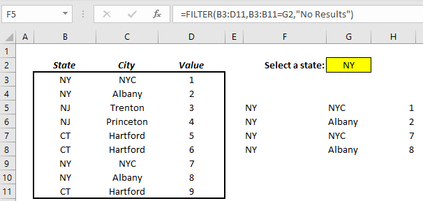
The example below shows a table on the left, an input cell, and the FILTER command in cell F5. In this case, the function is being used to look at the entire table (cells B3 through D11) and checking to see if the value in column B is the same as the value in cell G2.

Learn about Excel's FILTER Function

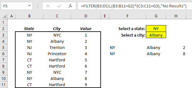
The formula for inclusion can use more complex approaches to check multiple values. This is done by using the multiplication operator as the “and” statement. The example below expands upon the first example by allowing the user to independently select both a state and a city.

IBM Planning Analytics Tips: Excel's FILTER Function

This functionality allows you to replicate Planning Analytics selector concepts into an existing spreadsheet.

IBM Planning Analytics, which TM1 is the engine for, is full of new features and functionality. Not sure where to start? Our team here at Revelwood can help. Contact us for more information at info@revelwood.com. And stay tuned for more Planning Analytics Tips & Tricks weekly in our Knowledge Center and in upcoming newsletters!

Read more IBM Planning Analytics Tips & Tricks:

IBM Planning Analytics Tips & Tricks: The Excel FORMULATEXT Function

IBM Planning Analytics Tips & Tricks: Learn the Excel CELL Formula

IBM Planning Analytics Tips & Tricks: New Excel Feature – Map Charts

Home » Excel tips & tricks » Page 2

Filed Under: IBM Planning Analytics Tips & Tricks Tagged With: Analytics, Excel, Excel tips & tricks, Financial Performance Management, IBM Cognos TM1, IBM Planning Analytics, Revelwood, TM1

IBM Planning Analytics Tips & Tricks: The Excel FORMULATEXT Function

June 16, 2020 by Lee Lazarow Leave a Comment

Tips & Tricks

Have you ever looked at a value on a report and wanted to know the formula that was used, even though you may not have access to the report? Have you ever wanted to easily include a formula as part of the report? Have you ever wanted to show people how complicated your calculation was as an attempt to get them to better appreciate you?

Well, all of this can be done in Excel with the use of a simple formula: FORMULATEXT.

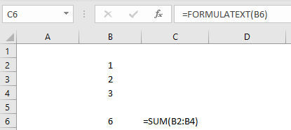
The FORMULATEXT function is used to return a formula as a string. The single parameter of the function is the cell to be converted to text.

The following example shows the use of the formula in cell C6.

IBM Planning Analytics Tips & Tricks: The Excel FORMULATEXT Function

Not only can you now show your co-workers how complicated your nested-if formulas have become, but you can also end those recurring nightmares about your middle school math teachers who always said “show me your work” (ok, maybe that’s just me).

IBM Planning Analytics, which TM1 is the engine for, is full of new features and functionality. Not sure where to start? Our team here at Revelwood can help. Contact us for more information at info@revelwood.com. And stay tuned for more Planning Analytics Tips & Tricks weekly in our Knowledge Center and in upcoming newsletters!

Read more IBM Planning Analytics Tips & Tricks:

IBM Planning Analytics Tips & Tricks: The Excel DATE Function

IBM Planning Analytics Tips & Tricks: New Excel Feature – XLOOKUP

IBM Planning Analytics Tips & Tricks: Excel’s IFS Function

Home » Excel tips & tricks » Page 2

Filed Under: IBM Planning Analytics Tips & Tricks Tagged With: Analytics, Excel, Excel tips & tricks, Financial Performance Management, IBM Cognos TM1, IBM Planning Analytics, Revelwood, TM1

IBM Planning Analytics Tips & Tricks: The Excel DATE Function

June 9, 2020 by Lee Lazarow Leave a Comment

Tips & Tricks

Many of you already know about Excel’s DATE function.  The function is used to create a date by defining specific values for the year, month and day.

DATE(2020,7,20) gives a result of 7/20/2020.

And some of you know that you can also use formulas to calculate a date.

If a value of 5 exists in cell C4 then

DATE(2020,7,20+C4) gives a result of 7/25/2020.

But did you know that the formula will also check for valid dates and, if needed, shift the month automatically?

DATE(2020,7,35) gives a result of 8/4/2020

(since there are not 35 days in July!)

and

DATE(2020,7,30+C4) gives the same result

Not only can this formula be used to calculate variable dates, but it will also ensure that you don’t incorrectly calculate a value that doesn’t exist on the calendar.  After all, we wouldn’t want Julius Caesar coming back to question our use of “his” month!

IBM Planning Analytics, which TM1 is the engine for, is full of new features and functionality. Not sure where to start? Our team here at Revelwood can help. Contact us for more information at info@revelwood.com. And stay tuned for more Planning Analytics Tips & Tricks weekly in our Knowledge Center and in upcoming newsletters!

Read more IBM Planning Analytics Tips & Tricks:

IBM Planning Analytics Tips & Tricks: Map Charts

IBM Planning Analytics Tips & Tricks: Sparklines

IBM Planning Analytics: Learn the Excel CELL Formula

Home » Excel tips & tricks » Page 2

Filed Under: IBM Planning Analytics Tips & Tricks Tagged With: Excel, Excel tips & tricks, Financial Performance Management, IBM Cognos TM1, IBM Planning Analytics, Revelwood, TM1

IBM Planning Analytics Tips & Tricks: Excel’s CONCAT and TEXTJOIN Functions

February 4, 2020 by Nina Inverso Leave a Comment

Tips & Tricks

Microsoft Excel has recently introduced a new version of the CONCATENATE function called CONCAT. The purpose is similar in that the new function still combines text from multiple ranges and/or strings. CONCAT will eventually replace CONCATENATE, but Microsoft has not released plans to sunset the original function to ensure compatibility with older versions of Excel.

The CONCAT function expects at least one text parameter value, with a maximum of 253 arguments. For example:

IBM Planning Analytics Tips & Tricks: CONCAT and TEXTJOIN Functions
=CONCAT(A1,B1,C1,D1,A2,B2,C2,D2)

returns “Tobeornottobe.” The new function also allows you to combine text ranges. For example:

=CONCAT(A1:D2)

returns a string consisting of the values in cells A1, B1, C1, D1, A2, B2, C2, and D2. In this case, “Tobeornottobe” will once again be returned.

Similarly, the TEXTJOIN function joins text from multiple ranges and/or strings but includes two additional parameters. These parameters allow you to specify the delimiter and determine if empty cells are ignored. For example:

=TEXTJOIN(“ ”, TRUE, A1:D2)

returns “To be or not to be,” whereas

=TEXTJOIN(“ ”, FALSE, A1:D2)

returns “To   be or not  to be.” In the last example, the spaces have been doubled wherever there are empty cells because the second parameter has been set to FALSE.

IBM Planning Analytics, which TM1 is the engine for, is full of new features and functionality. Not sure where to start? Our team here at Revelwood can help. Contact us for more information at info@revelwood.com. And stay tuned for more Planning Analytics Tips & Tricks weekly in our Knowledge Center and in upcoming newsletters!

Want to get our Planning Analytics Tips & Tricks delivered to your inbox every Tuesday? Sign up to get our weekly email of just the week’s tip!

Read related posts with Excel Tips & Tricks and using Excel with Planning Analytics:

IBM Planning Analytics Tips & Tricks: New Excel Feature – XLOOKUP

IBM Planning Analytics Tips & Tricks: Learn the Excel CELL Formula
IBM Planning Analytics Tips & Tricks: Recalculating Excel Worksheets

Home » Excel tips & tricks » Page 2

Filed Under: IBM Planning Analytics Tips & Tricks Tagged With: Analytics, Excel, Excel tips & tricks, Financial Performance Management, IBM Cognos TM1, IBM Planning Analytics, Nina Gordy, Revelwood, TM1

IBM Planning Analytics Tips & Tricks: Excel’s IFS Function

January 21, 2020 by Nina Inverso Leave a Comment

Tips & Tricks

While the IF function has been around for a while now, IFS is new to Excel. This function checks whether one or more conditions are met and then returns the value associated with the first TRUE condition. The main objective of IFS is to simplify an expression that would have previously required multiple nested IF functions.

The general format of the IFS function is

=IFS(Condition 1, Value if Condition 1 = TRUE, Condition 2, Value if Condition 2 = TRUE, Condition 3, Value if Condition 3 = TRUE)

The function can handle up to 127 different conditions, and only the first two parameters are required.

Here is an example using a sample Excel grid:

IBM Planning Analytics Tips & Tricks: Excel's IFS function
=IFS(A1>250,A2,B1>250,B2,C1>250,C2,D1>250,D2)

will return “Green” (the value of cell C2).

In older versions of Excel, this would be written as

=IF(A1>250,A2,IF(B1>250,B2,IF(C1>250,C2,IF(D1>250,D2))))

Multiple nested IF functions would previously be used to accomplish the same result.

IBM Planning Analytics, which TM1 is the engine for, is full of new features and functionality. Not sure where to start? Our team here at Revelwood can help. Contact us for more information at info@revelwood.com. And stay tuned for more Planning Analytics Tips & Tricks weekly in our Knowledge Center and in upcoming newsletters!

Want to get our Planning Analytics Tips & Tricks delivered to your inbox every Tuesday? Sign up to get our weekly email of just the week’s tip!

Read related posts with Excel Tips & Tricks and using Excel with Planning Analytics:

IBM Planning Analytics Tips & Tricks: New Excel Feature – XLOOKUP

IBM Planning Analytics Tips & Tricks: Learn the Excel CELL Formula
IBM Planning Analytics Tips & Tricks: Recalculating Excel Worksheets

Home » Excel tips & tricks » Page 2

Filed Under: IBM Planning Analytics Tips & Tricks Tagged With: Analytics, Excel tips & tricks, Financial Performance Management, FP&A, IBM Cognos TM1, IBM Planning Analytics, Nina Gordy, Revelwood, TM1

IBM Planning Analytics Tips & Tricks: Learn the Excel CELL Formula

December 3, 2019 by Lee Lazarow Leave a Comment

Tips & Tricks

Excel is, and always will be, a powerful tool for the financial team. With so much power, there are many great Excel formulas that rarely get used. I recently had a situation where I wanted to easily replicate a sheet and have each sheet use an MDX expression that referenced a different dimension name. I wanted to use a formula to determine the sheet name and used the CELL function.

The CELL function returns information about a specific cell within an Excel file. The syntax of the function is

CELL( info_type, reference ) 

The info_type defines the type of information to be returned and reference is associated with a specific cell. Some examples of info_type include “col” to define the column, “row” to define the row, “address” to define the cell refence and “filename” to return the full path and filename of the workbook and the worksheet.

The resulting format of the info_type called filename is

path[workbook.xlsm]sheetname

I took the approach of naming the sheet with the same name as the dimension. For example, one sheet was called “Account” and another sheet was called “Company.” By using a combination of the FIND function, the MID function and the TRIM function I was able to isolate the sheet name.

=TRIM(MID(CELL("filename",A1),FIND("]",CELL("filename"))+1,99))

I created this formula in cell B10 and then used the result within my MDX expression.

="{ TM1DRILLDOWNMEMBER( { ["&B10&"].[Orphans] }, ALL, RECURSIVE ) }"

This approach allows me to replicate an Active Form report by simply copying the entire sheet and then renaming the new sheet to be the same as the dimension name.

IBM Planning Analytics, which TM1 is the engine for, is full of new features and functionality. Not sure where to start? Our team here at Revelwood can help. Contact us for more information at info@revelwood.com. And stay tuned for more Planning Analytics Tips & Tricks weekly in our Knowledge Center and in upcoming newsletters!

Read more Excel-related tips & tricks:

IBM Planning Analytics Tips & Tricks: Recalculating Excel Worksheets

IBM Planning Analytics Tips & Tricks: Workarounds for Unsupported Excel Functions in TM1 Web

IBM Planning Analytics Tips & Tricks: New Excel Feature – XLOOKUP

Home » Excel tips & tricks » Page 2

Filed Under: IBM Planning Analytics Tips & Tricks Tagged With: Analytics, Budgeting, Budgeting Planning & Forecasting, Excel, Excel tips & tricks, Financial Performance Management, IBM Cognos TM1, IBM Planning Analytics, Revelwood, TM1

IBM Planning Analytics Tips & Tricks: New Excel Feature – XLOOKUP

October 29, 2019 by Lee Lazarow Leave a Comment

Tips & Tricks

Did you know Excel has a new feature called XLOOKUP?

For those of you who read these blogs regularly, you know that much of the focus is placed on IBM Planning Analytics Tips & Tricks.  However, I periodically also like to pass along new information about other planning and reporting aspects that impact your day-to-day tasks.

The VLOOKUP function has been around since Excel released version 1.0 in 1985. While VLOOKUP is one of the most widely used functions in Excel, there are some limitations:

  • Finding an “approximate” match
  • How to easily add columns in the search range
  • Define a search value in the middle of the range (e.g., not as the first column)
  • Starting a search at the bottom of your list without having to re-sort the data table

Microsoft recently announced the addition of a new function called XLOOKUP that is designed to simplify the lookup approach while merging functions such as VLOOKUP, HLOOKUP, INDEX and MATCH into a single function. The function is written as:

XLOOKUP(lookup_value,lookup_array,return_array,[match_mode],[search_mode])

lookup value: the value you are looking for (the same as VLOOKUP)

lookup_array: the lookup column (the same as VLOOKUP)

return_array: the results column (the same as VLOOKUP)

match_mode: This is an optional parameter that determines what kind of match to find.  The options include an exact match, an exact match or the next smaller item, an exact match or the next larger item, or a wildcard search.

search_mode: This is an optional parameter that allows you to determine whether the search happens from first-to-last or from last-to-first.

This new approach will make searching easier by not having to repeatedly modify your search table while also adding new functionality for tasks such as looking up a tax rate within a range of results.

There are many instances where the inclusion of Excel functions can help further your analytics. XLOOKUP is just one example.

IBM Planning Analytics, which TM1 is the engine for, is full of new features and functionality. Not sure where to start? Our team here at Revelwood can help. Contact us for more information at info@revelwood.com. And stay tuned for more Planning Analytics Tips & Tricks weekly in our Knowledge Center and in upcoming newsletters!

Home » Excel tips & tricks » Page 2

Filed Under: IBM Planning Analytics Tips & Tricks Tagged With: Analytics, Beyond Budgeting, Budgeting, Budgeting Planning & Forecasting, Excel, Excel tips & tricks, Financial Performance Management, IBM Cognos TM1, IBM Planning Analytics, new excel feature, Planning & Forecasting, Planning & Reporting, Revelwood, TM1, XLOOKUP

  • « Go to Previous Page
  • Page 1
  • Page 2

Footer

Revelwood Overview

Revelwood helps finance organizations close, consolidate, plan, monitor and analyze business performance. As experts in solutions for the Office of Finance, we partner with best-in-breed software companies by applying best practices guidance and our pre-configured applications to help businesses achieve their full potential.

EXPERTISE

  • Workday Adaptive Planning
  • IBM Planning Analytics
  • BlackLine

ABOUT

  • Who We Are
  • What We Do
  • How We Help
  • How We Think
  • Privacy

CONNECT

World Headquarters

Florham Park, NJ | 201 984 3030

European Headquarters

London & Edinburgh | +44 (0)131 240 3866

Latin America Office

Miami, FL | 201 987 4198

Email
info@revelwood.com

Copyright © 2025 · Revelwood Inc. All rights reserved. Revelwood® and the Revelwood logo are registered marks of Revelwood Inc.