The SWITCH function in Excel evaluates a condition and then provides a result based on that condition. This function is similar to a SQL CASE statement and allows for up to 126 potential results.
The syntax of the SWITCH function is:
=SWITCH(expression, value1, result1, value2, result2, …, no match value)
- The Expression is the value to be analyzed. This can be any formula, including another Excel formula.
- The resulting value can be a text string or a decimal.
- Result1 is the value to be referenced/matched. This is the result of the expression.
- Value1 is the replacement (switch) value.
- The “no match value” is the result if no matches are found.
Here is an example of the formula:
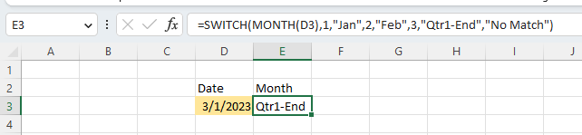
This example returns the month short name for January and February but will return ‘Qtr1-End’ for March. If no match is found, the text value “No Match” will be returned.
This approach will allow you to merge IF statements and LOOKUP statements into a single command.
IBM Planning Analytics, which TM1 is the engine for, is full of new features and functionality. Not sure where to start? Our team here at Revelwood can help. Contact us for more information at info@revelwood.com. And stay tuned for more Planning Analytics Tips & Tricks weekly in our Knowledge Center and in upcoming newsletters!
Read more about visualizations in IBM Planning Analytics:
IBM Planning Analytics Tips & Tricks: Excel TEXT Function
Top Three IBM Planning Analytics Tips & Tricks Posts – 2023
IBM Planning Analytics Tips & Tricks: Using the Subset Editor in Planning Analytics Workspace