Excel tips & tricks

IBM Planning Analytics Tips & Tricks: PAW “Spacers”

March 19, 2024 by Lee Lazarow

Have you ever created an exploration in IBM Planning Analytics Workspace (PAW) that contains a lot of data and wish that you could separate the information? PAW allows you to insert blank rows and columns called “spacers” into your exploration.

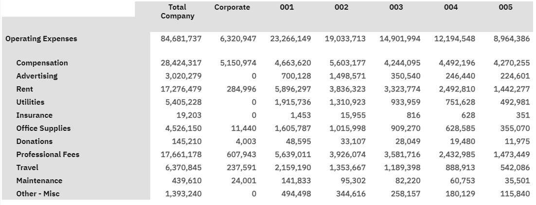
Here is an example of a grid that shows expenses by company:

A screenshot of a graph

Description automatically generated

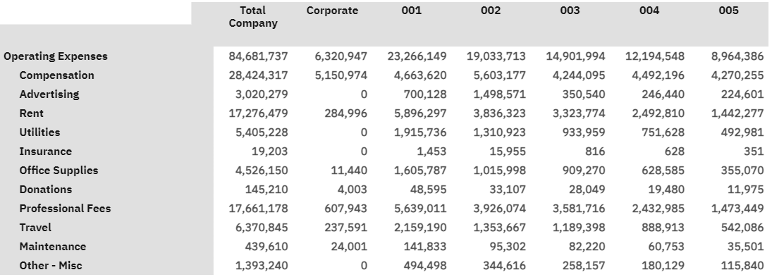
This subset of data is not very large, but it’s somewhat difficult to differentiate the totals from the details within the grid. This is an example where spacers can help.

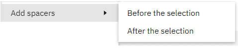
You can insert a space by simply right-clicking on the area where you want to insert the blank row or column and then selecting the option to “Add spacers.” You can insert the spacer before or after the area that was clicked.

Here is the same example after inserting a blank row that separates the total expense value from the account values:

A screenshot of a computer screen

Description automatically generated

From there, we can adjust the size of the spacer and update the formatting of the top row to make the total values stand out.

This approach will help make it easier for you to create easy-to-read explorations for your users.

IBM Planning Analytics, which TM1 is the engine for, is full of new features and functionality. Not sure where to start? Our team here at Revelwood can help. Contact us for more information at info@revelwood.com. And stay tuned for more Planning Analytics Tips & Tricks weekly in our Knowledge Center and in upcoming newsletters!

IBM Planning Analytics Tips & Tricks: Excel’s ROUND Function

March 5, 2024 by Lee Lazarow

Most standard financial reports round to some form of a large value. For example, the report may show numbers in millions or rounded to the nearest 100,000.

This is done in Excel via the ROUND function. The function has two parameters:

=ROUND(number, num_digits)

The number defines the initial value to be rounded
The number of digits determines how many digits to round the number

Here is an example of a large value with various rounding results:

Table

Description automatically generated

But did you know that you have a variety of options for the number of digits?

A positive value rounds to the nearest applicable decimal
A zero value rounds to the nearest integer
A negative value rounds to the left of the decimal point

Here is the same example using negative rounding:

Graphical user interface, table, Excel

Description automatically generated

This approach could also be used to round to the nearest thousand (-3) or the nearest million (-6).

In addition, Excel offers two other options: ROUNDUP and ROUNDDOWN.

ROUNDUP will always round away from zero (e.g., round up)
ROUNDDOWN will always round toward from zero (e.g., round down)

By using a combination of the appropriate ROUND function and a positive/negative number, you can ensure that all your reports show the values you want users to see.

IBM Planning Analytics Tips & Tricks: Excel’s XMATCH Function

May 17, 2022 by Lee Lazarow

Have you ever wanted to search a list and define the position where it appears in the list? Maybe you want to know how many sales reps exceeded their quota or want to define how many products cost more than an approved purchase price. This information can be calculated using Excel’s XMATCH function.

The XMATCH function is used to determine the number position of an item in a list.

The syntax of the function is:

=XMATCH (lookup_value, lookup_array, [match_mode], [search_mode])

Lookup_value
- This is required
Lookup_array
- This is required
Match_mode
- This is optional
- This determines whether you are looking for an exact match or whether you want to look for the next smallest or largest item
Search_mode
- This is optional
- This defines various approaches for top-to-bottom or bottom-to-top searches

The following example shows how to determine the number of sales reps that exceeded a sales quota. The lookup value is defined as the quota amount, the lookup array defines a list of sales amounts, and the match mode defines “Exact match or next largest item.”

This formula can be used independently to find vales within a list and can also be combined with other formulas such as COUNT to define the “not exceeded” values.

IBM Planning Analytics Tips & Tricks: Excel Workbook Stats

May 3, 2022 by Lee Lazarow

Have you ever wanted to know details about your existing worksheet or workbook such as the number of cells that contain data or the number of total sheets? In 2021, Microsoft Excel introduced a feature called Workbook Statistics that will provide details about your file.

The Workbook Statistics icon is found within the proofing area of the Review ribbon.

When the icon is clicked, a window appears to show details about the sheet. The following statistics are shown:

Worksheet level

End of sheet / Last cell
Number of Cells with Data
Number of Tables
Number of PivotTables
Number of Formulas
Number of Charts
Number of Images
Number of Form Controls
Number of Objects
Number of Comments
Number of Notes

Workbook level

Number of Sheets
Number of Cells with Data
Number of Tables
Number of PivotTables
Number of Formulas
Number of Charts
Number of External Connections
Number of Macros

Here is an example of a simple sheet that contains some input cells, some calculations, and a header row:

Not only will these details help you with generic Excel related questions, but the “end of sheet” and “cells with data” details can also assist when reviewing your dynamic reporting setups.

IBM Planning Analytics Tips & Tricks: Excel DATE Function Updated

August 17, 2021 by Lee Lazarow Leave a Comment

Some of you may remember an Excel feature that I posted about last year which explained how the DATE function will convert invalid dates into real ones. For example, DATE(2020,7,35) will be converted to August 4, 2020 since there are not 35 days in July.

Here is where the fun begins!

This week includes the 20^th day of the month of August
August is the 8^th month of this year, which is also the 20^th month of last year
Last year was 2020

Put this all together and we have a special event happening this week …

On August 20, 2021,

the resulting date will be 20/20/2020

And if we take it a step further …

At 8:20p and 20 seconds on 8/20/2021,

the resulting time will be 20:20:20 on 20/20/20

This is why we love Excel!

Workday Adaptive Planning Tips & Tricks: Excel Substitute

March 3, 2021 by Michelle Song Leave a Comment

We have something different for today’s Workday Adaptive Planning Tips & Tricks post – an Excel tip! Our Adaptive Planning users also use Excel, so we thought they’d find this helpful.

Have you ever wanted to get rid of spaces in some of your Excel cells? Maybe you do not want a cell to have separate words and instead want to use an underscore character. Or maybe you are in a situation where you want to adjust a prefix for a certain range of cells. You can use Excel’s find and replace functionality, but this approach could lead to a time consuming effort if you want to pick and choose the cells where it applies.

Excel’s SUBSTITUTE function can help you solve this problem. The SUBSTITUTE function is used to find a specific set of characters and replace it with something else while also giving you the ability to define details within cells.

The syntax of the function is:

=SUBSTITUTE (text, old_text, new_text)

text
- This is the source that will be changed; this is typically a cell reference.
old_text
- This is the subtext that will be replaced.
new_text
- This is what will replace the old subtext

If the cell in A5 consists of “Happy Birthday” then it can be updated to “Happy_Birthday” via the following:

=SUBSTITUTE (A5, “ “, “_”)

In addition, the parameter that defines the new text can also be a cell reference. This gives you the ability to quickly change the results of a large set of data by simply updating a single cell.

This approach will allow you to quickly find and replace characters within specific cells instead of having to manually go through a set of cells via Excel’s find and replace functionality.

The team at Revelwood has been recognized by Adaptive for its thought leadership in the space, commitment to its Adaptive Insights practice, and its rapid achievements of milestones. Visit Revelwood’s Knowledge Center for our Adaptive Insights Tips & Tricks or sign up here to get our Adaptive Insights Tips & Tricks delivered directly to your inbox. Not sure where to start with Adaptive Insights? Our team here at Revelwood can help! Contact us info@revelwood.com for more information.

IBM Planning Analytics Tips & Tricks: Manipulating Text in Excel

February 2, 2021 by Lee Lazarow Leave a Comment

Have you ever wanted to manipulate text within Excel? Excel has a series of functions that allow you to parse text strings based on whether you want to reference the left, the right, or the middle of the cell contents.

For example, assume cell A2 contains the text “Planning Analytics”. The functions LEFT and RIGHT will allow you to view characters at the start of the string or at the end of the string.

=LEFT(A2,3) will give a result of “Pla”

=RIGHT(A2,3) will give a result of “ics”

The function MID will allow you to look within the string by defining both a starting point and the number of characters in the result.

=MID(A2,3,3) will give a result of “ann”

But what if you didn’t know the number of characters? You can use functions to find a specific set of characters and to determine the overall length of the string.

=FIND(“A”,A2)-1 will give a result of “9”, which signifies that the string begins at the 9^th character

=LEN(A2) will give a result of “18”, which signifies that the string contains 18 total characters

You can then put these pieces together to find a specific set of data, such as the second word in the string. Assuming that D6 contains the LEN function and D5 contains the FIND function:

=RIGHT(A2,D6-D5) will give a result of “Analytics”

These Excel functions will allow you to quickly parse out pieces of a text string which can then be used in your spreadsheets.

IBM Planning Analytics Tips & Tricks: Excel’s NETWORKDAYS Function

January 26, 2021 by Lee Lazarow Leave a Comment

Have you ever wanted to define the number of working days between two calendar dates? Do you define “working days” simply as non-weekend days or do you also include holidays? Did you know that you can calculate this information using Excel’s NETWORKDAYS function?

The NETWORKDAYS function is used to determine the number of whole working days between start_date and end_date. Working days are defined as the exclusion of weekends, which in essence computes the number of Mondays through Fridays. The function also includes an optional parameter to exclude holidays and any other specific non-working days.

The syntax of the function is:

NETWORKDAYS (start_date, end_date, [holidays])

Start_date: This is required
End_date: This is required
Holidays: This is optional
- This consists of a range of one or more dates to be excluded from the calendar. The list entails a range of cells that contains the dates.

Note: All dates are entered in date format or in serial number format

This information can be used to help calculate any/all of the following pieces of your model:

Benefit accruals and eligibility
Ratios such as “Revenue per day” or “Units per day”
Days remaining for end-of-service dates
Anything else that requires the number of days within the formula

IBM Planning Analytics Tips & Tricks: Excel TYPE Function

January 12, 2021 by Lee Lazarow Leave a Comment

Have you ever referenced a list in Excel and needed to know whether each value was a number or a string? This may be required when another function depends on the type of value in each cell.

Excel has a function called TYPE that will give you this information. The function contains a single parameter, which is simply the cell you want to check. The formula will output a number that defines the type of value such as number, text, logical value or an error.

Here are results from four iterations of the TYPE formula:

IBM Planning Analytics Tips & Tricks: Excel Type

You can then use the type result within an IF statement to perform various functions.

The TYPE function will not determine whether a cell contains a formula. TYPE only determines the type of the resulting, or displayed, value. If value is a cell reference to a cell that contains a formula, TYPE returns the type of the formula’s resulting value.

This approach will help you when determining the use of IBM Planning Analytics formulas such as DBS vs. DBSS.

IBM Planning Analytics Tips & Tricks: PAW “Spacers”

Read more IBM Planning Analytics Tips & Tricks:

IBM Planning Analytics Tips & Tricks: Excel’s ROUND Function

Read more IBM Planning Analytics Tips & Tricks:

IBM Planning Analytics Tips & Tricks: Excel’s XMATCH Function

Read more Excel Tips & Tricks:

IBM Planning Analytics Tips & Tricks: Excel Workbook Stats

Read more Excel Tips & Tricks:

IBM Planning Analytics Tips & Tricks: Excel DATE Function Updated

Read more Excel tips from our IBM Planning Analytics team:

Workday Adaptive Planning Tips & Tricks: Excel Substitute

Read more Workday Adaptive Planning Tips & Tricks:

IBM Planning Analytics Tips & Tricks: Manipulating Text in Excel

Read more Excel tips in our IBM Planning Analytics Tips & Tricks series:

IBM Planning Analytics Tips & Tricks: Excel’s NETWORKDAYS Function

Read more Excel tips in our IBM Planning Analytics Tips & Tricks series:

IBM Planning Analytics Tips & Tricks: Excel TYPE Function

Read more Excel tips & tricks:

Revelwood Overview

EXPERTISE

ABOUT

CONNECT

Excel tips & tricks

Read more IBM Planning Analytics Tips & Tricks:

Read more IBM Planning Analytics Tips & Tricks:

Read more Excel Tips & Tricks:

Read more Excel Tips & Tricks:

Read more Excel tips from our IBM Planning Analytics team:

Read more Workday Adaptive Planning Tips & Tricks:

Read more Excel tips in our IBM Planning Analytics Tips & Tricks series:

Read more Excel tips in our IBM Planning Analytics Tips & Tricks series:

Read more Excel tips & tricks:

Footer

Revelwood Overview

EXPERTISE

ABOUT

CONNECT